
Left-skewed histograms have a longer tail on the left, with the median typically greater than the mean, while right-skewed histograms have a longer tail on the right, with the mean typically greater than the median.
When analyzing histograms, understanding left and right skewness is essential. A left skewed histogram shows a longer tail on the left, while a right skewed one has its tail extending to the right. These differences in distribution can significantly affect your data interpretation. But how do these patterns influence the relationship between mean and median? The nuances behind skewness could change how you approach your analysis. Let's explore this further.
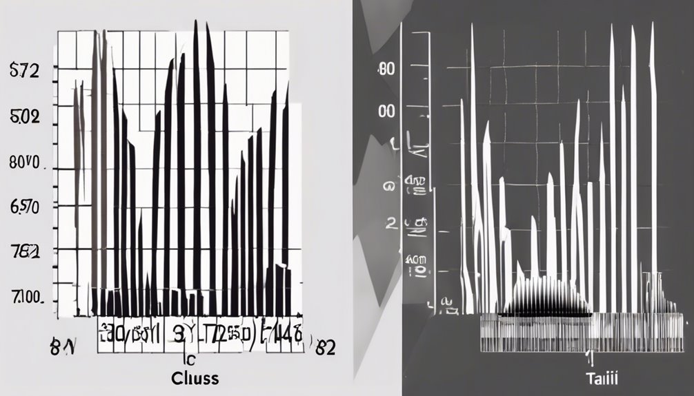
Understanding Histogram Basics

Histograms are a powerful tool for visualizing data distribution, especially when you want to see how values are spread across different ranges. They display data in intervals, or bins, allowing you to quickly grasp the frequency of data points within each range.
When creating a histogram, choose appropriate bin sizes; too large can obscure details, while too small may create noise. Each bar represents the count of data points falling within that bin, making it easy to identify patterns or trends.
You'll find histograms particularly useful for understanding the overall shape of your dataset, whether it's uniform, bimodal, or exhibits other characteristics. By interpreting these visuals, you can make informed decisions based on your data's distribution.
Defining Left Skewed Distributions
When analyzing data distributions, you might come across the term "left skewed" or "negatively skewed." This refers to a distribution where the tail on the left side is longer or fatter than the right side.
In a left skewed distribution, most data points cluster toward the higher end of the scale, with fewer values dragging the mean down. This means that the median is typically higher than the mean, reflecting that larger values dominate.
You'll often see this in situations where there's a natural limit on the higher end, but a wide range of lower values. Understanding left skewed distributions is crucial, as they can affect the interpretation of your data and influence statistical analysis.
Characteristics of Right Skewed Distributions

Right skewed distributions, often called positively skewed, occur when the tail on the right side is longer or fatter than on the left. In these distributions, most of your data points cluster on the lower end, with a few higher values stretching the tail.
You'll notice that the mean is typically greater than the median, as those higher values pull the average up. This can lead to an underestimation of central tendency if you're only looking at the mean.
Additionally, right skewed distributions often arise in real-world scenarios like income levels, where a small number of individuals earn significantly more than the majority.
Recognizing these characteristics helps you analyze data more effectively.
Visual Representation of Skewness
Understanding the visual representation of skewness is vital for interpreting data distributions accurately. When you look at a histogram, pay attention to the shape. In a left-skewed distribution, the tail points to the left, indicating that a majority of the data is concentrated on the right.
Conversely, a right-skewed distribution has its tail extending to the right, showcasing that most values are lower, with a few high outliers. Recognizing these patterns helps you draw conclusions about the underlying data.
Additionally, note the peak's position; it often shifts in relation to the skewness. By grasping these visual cues, you can better analyze trends, make predictions, and understand the overall data landscape effectively.
Implications of Left Skewness in Data Analysis

Although left skewness might seem less common than right skewness, it has significant implications for data analysis.
When you encounter a left-skewed distribution, it often indicates that most of your data points cluster on the higher end, with a few low outliers pulling the mean down. This can affect your statistical measures; for instance, the mean will be less representative of the dataset than the median.
You might also want to reconsider how you interpret trends or make predictions, as left skewness can suggest underlying issues or anomalies in your data.
Recognizing this skewness helps you to adjust your analysis methods, ensuring you draw accurate conclusions and make informed decisions based on the data at hand.
Impact of Right Skewness on Interpretation
Left skewness highlights how data can be pulled by outliers, but right skewness presents its own set of challenges for interpretation.
When you're analyzing right-skewed data, you might find the mean significantly higher than the median. This difference can lead to misconceptions if you don't account for it. For instance, a few high values can distort your understanding of the overall dataset.
You may also encounter difficulties in making predictions, as right-skewed distributions often suggest that most values cluster at lower ranges with a long tail extending to the right.
It's crucial to recognize these patterns to avoid overestimating central tendencies and make informed decisions based on accurate data interpretations. Always consider the skewness before drawing conclusions.
Examples of Left Skewed Data

Skewness can significantly influence data interpretation, and left skewed data offers unique insights into certain real-world scenarios.
For example, consider income distribution in a community where a majority earn below the average, but a few individuals earn considerably more. This situation results in a left skewed histogram.
Another instance is the age at retirement; most people retire around a certain age, but a few may retire much earlier, creating a left skew.
Additionally, test scores can demonstrate left skewness if most students score high but a few struggle significantly.
In these cases, understanding the left skew helps you identify trends and anomalies, guiding decisions and strategies in areas like policy-making, education, and economic analysis.
Examples of Right Skewed Data
In contrast to left skewed data, right skewed data reveals a different set of patterns and implications.
You often encounter right skewed data in scenarios like income distribution, where a small number of individuals earn significantly more than the majority.
Another example is the age at retirement; while most people retire around a certain age, some work much longer, creating a tail on the right.
Similarly, in real estate, home prices can be right skewed, with a few high-value properties pushing the average upwards.
Exam scores can also exhibit right skewness, as many students score lower with a few excelling greatly.
Recognizing these examples helps in understanding the nature of right skewed distributions in various contexts.
Analyzing Skewness in Real-World Scenarios
How do real-world scenarios illustrate the concept of skewness?
You can see skewness in various fields, from finance to healthcare. For instance, income distribution often shows right skewness, as a small number of individuals earn significantly higher wages than the majority.
In contrast, ages at retirement illustrate left skewness; most people retire around a certain age, but a few retire much earlier, creating a tail on the left.
Understanding these examples helps you grasp the implications of skewness in data analysis. Recognizing which way the data skews can guide your decisions, whether you're evaluating business strategies or interpreting survey results.
Techniques for Addressing Skewed Data
When dealing with skewed data, you can employ several techniques to enhance your analysis and ensure more accurate results.
First, consider transforming your data using logarithmic, square root, or cube root transformations. These methods can reduce skewness and make your data more normally distributed.
Second, you might want to use robust statistical measures, like the median or interquartile range, which are less affected by outliers.
Third, consider applying non-parametric tests, as they don't assume normality.
Lastly, data binning can help smooth out the skewness by grouping data into ranges.
Conclusion
In conclusion, understanding left and right skewed histograms is essential for accurate data interpretation. By recognizing the characteristics of each distribution, you can make informed decisions about the statistical techniques to use. Whether you're analyzing income data or test scores, identifying skewness helps you grasp the underlying patterns and relationships between mean and median. Embracing these concepts will enhance your analytical skills and enable you to draw more meaningful insights from your data.